Overview

This project was initiated as the final assignment for Bangkit Academy 2024. The goal of the assignment was to develop an Android application that utilized both Machine Learning and Cloud Computing. Each team had to include students from all three learning paths: Machine Learning, Cloud Computing, and Mobile Development. Since I took the Machine Learning path, this page mainly discusses my experience doing the machine learning side of the project.

During our team’s first online meeting, we discussed several great ideas. However, we soon realized some constraints, such as limited time and resources. Therefore, we decided to create a relatively simple waste-sorting application that used widely available open-source data, which we eventually named “DaurYuk: Sorting Waste for a Sustainable Future.”

Objectives

Formally speaking, this project aimed to address improper waste management in Indonesia, which can lead to increased pollution, depletion of natural resources, and negative impacts on ecosystems and biodiversity. However, as I’m writing this, I realize that solving this issue requires more involvement from the government rather than relying on a single application alone. Still, this application is intended to help Indonesian people learn to sort their waste so they can decide what to do with it, such as recycling or upcycling, instead of letting everything end up in a garbage dumpster.

Methods & Tools

Phase 1: Base Model MobileNetV3large

Data Preparation

The main data is sourced from this Kaggle dataset named RealWaste Image Classification. It contains images categorized into nine classes, with the following number of samples for each:

1. Cardboard — 461
2. Food Organics — 411
3. Glass — 420
4. Metal — 790
5. Miscellaneous Trash — 495
6. Paper — 500
7. Plastic — 921
8. Textile Trash — 318
9. Vegetation — 436

Model Development and Training

In this project, we decided to use a transfer learning approach by utilizing a pretrained model, specifically MobileNetV3Large, to address our problem. We then added additional dense and dropout layers to improve convergence on our dataset. Subsequently, the model was compiled with Adam optimizer and Categorical Loss Entropy loss function.

import tensorflow as tf
from tensorflow.keras.applications import MobileNetV3Large
from tensorflow.keras import layers
from tensorflow.keras.models import Model
from tensorflow.keras.optimizers import Adam

pretrained_model = MobileNetV3Large(
    input_shape=(224, 224, 3),
    include_top=False,   
    weights='imagenet',
    pooling='avg'        
)

pretrained_model.trainable = False

# Define model structure
inputs = pretrained_model.input
x = pretrained_model.output

# Add custom classification layers
x = layers.Dense(512, activation='relu')(x)
x = layers.Dropout(0.2)(x)
x = layers.Dense(256, activation='relu')(x)
x = layers.Dropout(0.2)(x)
outputs = layers.Dense(9, activation='softmax')(x)

# Build the model
model = Model(inputs=inputs, outputs=outputs, name="MobileNetV3_TransferLearning")

# Compile the model
model.compile(
    optimizer=Adam(learning_rate=1e-4),
    loss='categorical_crossentropy',
    metrics=['accuracy']
)

By utilizing two callback functions: Reduce Learning Rate and Early Stopping, the training process was completed at the 50th epoch with a learning rate of 1e-5.

from tensorflow.keras.callbacks import ReduceLROnPlateau, EarlyStopping

reduce_lr = ReduceLROnPlateau(monitor='val_loss', factor=0.5, patience=5, min_lr=0.00001)
early_stopping = EarlyStopping(monitor='val_loss', mode='min', patience=15, restore_best_weights=True, verbose=1)

history = model.fit(
    train_images,
    steps_per_epoch=len(train_images),
    validation_data=val_images,
    validation_steps=len(val_images),
    epochs=100,
    callbacks=[reduce_lr, early_stopping]
)

Epoch 1/100
96/96 [==============================] - 41s 245ms/step - loss: 1.7364 - accuracy: 0.3956 - val_loss: 1.0822 - val_accuracy: 0.6539 - lr: 1.0000e-04
Epoch 2/100
96/96 [==============================] - 16s 169ms/step - loss: 1.0444 - accuracy: 0.6370 - val_loss: 0.8007 - val_accuracy: 0.7461 - lr: 1.0000e-04
Epoch 3/100
96/96 [==============================] - 24s 246ms/step - loss: 0.8168 - accuracy: 0.7175 - val_loss: 0.6694 - val_accuracy: 0.7737 - lr: 1.0000e-04
Epoch 4/100
96/96 [==============================] - 16s 167ms/step - loss: 0.6727 - accuracy: 0.7590 - val_loss: 0.6030 - val_accuracy: 0.7974 - lr: 1.0000e-04
Epoch 5/100
96/96 [==============================] - 16s 168ms/step - loss: 0.5862 - accuracy: 0.7869 - val_loss: 0.5643 - val_accuracy: 0.7987 - lr: 1.0000e-04
...
Epoch 46/100
96/96 [==============================] - 16s 167ms/step - loss: 0.0313 - accuracy: 0.9957 - val_loss: 0.3911 - val_accuracy: 0.8816 - lr: 1.0000e-05
Epoch 47/100
96/96 [==============================] - 16s 169ms/step - loss: 0.0289 - accuracy: 0.9957 - val_loss: 0.3903 - val_accuracy: 0.8816 - lr: 1.0000e-05
Epoch 48/100
96/96 [==============================] - 16s 169ms/step - loss: 0.0289 - accuracy: 0.9967 - val_loss: 0.3904 - val_accuracy: 0.8816 - lr: 1.0000e-05
Epoch 49/100
96/96 [==============================] - 18s 192ms/step - loss: 0.0285 - accuracy: 0.9970 - val_loss: 0.3882 - val_accuracy: 0.8816 - lr: 1.0000e-05
Epoch 50/100
96/96 [==============================] - ETA: 0s - loss: 0.0240 - accuracy: 0.9993Restoring model weights from the end of the best epoch: 35.
96/96 [==============================] - 16s 169ms/step - loss: 0.0240 - accuracy: 0.9993 - val_loss: 0.3918 - val_accuracy: 0.8803 - lr: 1.0000e-05
Epoch 50: early stopping

Model Evaluation

In this first phase, the model achieved an accuracy of 85%. It was already a satisfactory result, according to our machine learning project advisor. However, since we set a target of more than 90% in our project plan, we decided to optimize the model until it reached the desired result.

results = model.evaluate(test_images, verbose=0)

print("    Test Loss: {:.5f}".format(results[0]))
print("Test Accuracy: {:.2f}%".format(results[1] * 100))

    Test Loss: 0.49703
Test Accuracy: 84.96%

Phase 2: Unfreeze 50% of MobileNetV3Large’s Layers

Model Development and Training

In the earlier phase, we concluded that the model may not have been trained well to our data. The model was unable to learn much new information, since every layer of the base model was frozen or untrainable. Therefore, in this phase, we tried unfreezing half of the base model’s layers.

import tensorflow as tf
from tensorflow.keras.applications import MobileNetV3Large
from tensorflow.keras import layers
from tensorflow.keras.models import Model
from tensorflow.keras.optimizers import Adam

pretrained_model = MobileNetV3Large(
    input_shape=(224, 224, 3),
    include_top=False,   
    weights='imagenet',
    pooling='avg'        
)

layers_count = len(pretrained_model.layers)
for i in range(int(layers_count*0.5)):
    pretrained_model.layers[i].trainable = False
# for layer in pretrained_model.layers:
#     layer.trainable = False

# Define model structure
inputs = pretrained_model.input
x = pretrained_model.output

# Add custom classification layers
x = layers.Dense(512, activation='relu')(x)
x = layers.Dropout(0.2)(x)
x = layers.Dense(256, activation='relu')(x)
x = layers.Dropout(0.2)(x)
outputs = layers.Dense(9, activation='softmax')(x)

# Build the model
model = Model(inputs=inputs, outputs=outputs)

# Compile the model
model.compile(
    optimizer=Adam(learning_rate=1e-4),
    loss='categorical_crossentropy',
    metrics=['accuracy']
)

Still using the same callback functions, the model finished the training process at the 33rd epoch with a learning rate of 2.5e-5.

from tensorflow.keras.callbacks import ReduceLROnPlateau, EarlyStopping

reduce_lr = ReduceLROnPlateau(monitor='val_loss', factor=0.5, patience=5, min_lr=0.00001)
early_stopping = EarlyStopping(monitor='val_loss', mode='min', patience=15, restore_best_weights=True, verbose=1)

history = model.fit(
    train_images,
    steps_per_epoch=len(train_images),
    validation_data=val_images,
    validation_steps=len(val_images),
    epochs=100,
    callbacks=[reduce_lr, early_stopping]
)

Epoch 1/100
90/90 [==============================] - 32s 214ms/step - loss: 1.5568 - accuracy: 0.4595 - val_loss: 1.2065 - val_accuracy: 0.5274 - lr: 1.0000e-04
Epoch 2/100
90/90 [==============================] - 17s 194ms/step - loss: 0.7099 - accuracy: 0.7611 - val_loss: 0.9753 - val_accuracy: 0.6358 - lr: 1.0000e-04
Epoch 3/100
90/90 [==============================] - 18s 202ms/step - loss: 0.4199 - accuracy: 0.8565 - val_loss: 0.9506 - val_accuracy: 0.6537 - lr: 1.0000e-04
Epoch 4/100
90/90 [==============================] - 19s 215ms/step - loss: 0.2589 - accuracy: 0.9200 - val_loss: 0.7932 - val_accuracy: 0.7284 - lr: 1.0000e-04
Epoch 5/100
90/90 [==============================] - 19s 210ms/step - loss: 0.1790 - accuracy: 0.9418 - val_loss: 0.7439 - val_accuracy: 0.7484 - lr: 1.0000e-04
...
Epoch 29/100
90/90 [==============================] - 18s 195ms/step - loss: 0.0036 - accuracy: 0.9996 - val_loss: 0.5579 - val_accuracy: 0.8884 - lr: 2.5000e-05
Epoch 30/100
90/90 [==============================] - 19s 214ms/step - loss: 0.0039 - accuracy: 0.9993 - val_loss: 0.5523 - val_accuracy: 0.8874 - lr: 2.5000e-05
Epoch 31/100
90/90 [==============================] - 18s 200ms/step - loss: 0.0031 - accuracy: 0.9996 - val_loss: 0.5440 - val_accuracy: 0.8916 - lr: 2.5000e-05
Epoch 32/100
90/90 [==============================] - 17s 194ms/step - loss: 0.0022 - accuracy: 0.9996 - val_loss: 0.5469 - val_accuracy: 0.8926 - lr: 2.5000e-05
Epoch 33/100
90/90 [==============================] - ETA: 0s - loss: 0.0023 - accuracy: 0.9996Restoring model weights from the end of the best epoch: 18.
90/90 [==============================] - 19s 208ms/step - loss: 0.0023 - accuracy: 0.9996 - val_loss: 0.5491 - val_accuracy: 0.8916 - lr: 2.5000e-05
Epoch 33: early stopping

Model Evaluation

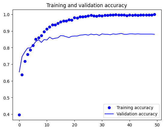
As the results show, this approach managed to attain higher accuracy than before. However, when we look at the training and validation accuracy, it appears to be overfitting, with the training accuracy close to 100%. This means that the model may not perform well on new, unseen data.

results = model.evaluate(test_images, verbose=0)

print("    Test Loss: {:.5f}".format(results[0]))
print("Test Accuracy: {:.2f}%".format(results[1] * 100))

    Test Loss: 0.51541
Test Accuracy: 88.12%

Phase 3: Address the Overfitting

Data Gathering

One technique to deal with the overfitting of the model is adding new data. We therefore made the decision to look up additional waste image data. We ultimately used the Garbage Classification data, which has twelve classifications:

1. Battery — 945
2. Biological — 985
3. Brown Glass — 607
4. Cardboard — 891
5. Clothes — 5325
6. Green Glass — 629
7. Metal — 769
8. Paper — 1050
9. Plastic — 865
10. Shoes — 1977
11. Trash — 697
12. White Glass — 755

Data Preprocessing

Since the two datasets had different class labels, we needed to combine and omit some of the classes in the dataset. We merged the original dataset into only 8 classes to achieve greater data variety while still considering the same waste disposal method, which resulting the final dataset below:

1. Cardboard — 1352
2. Food Organics — 1832
3. Glass — 2431
4. Metal — 1559
5. Miscellaneous Trash — 1440
6. Paper — 1550
7. Plastic — 1786
8. Textile trash — 1818

From this dataset, we can observe a slight imbalance, which can be calculated using the ratio between the class with the most samples and the class with the fewest samples. In this case, the largest class (Glass: 2431 samples) compared to the smallest class (Cardboard: 1352 samples) gives an imbalance ratio of approximately 1.8 : 1. This number of imbalance is still manageable, but to further reduce the risk of bias during training, we applied oversampling using SMOTE (Synthetic Minority Oversampling Technique).

import numpy as np
import pandas as pd
import os
from pathlib import Path

from tensorflow.keras.preprocessing.image import ImageDataGenerator
from tensorflow.keras.preprocessing.image import array_to_img

from imblearn.over_sampling import SMOTE

# Oversampling ---

# load data from the dataframe
load_gen = ImageDataGenerator()
smote_gen = load_gen.flow_from_dataframe(
  dataframe=train_df,
  x_col='Filepath',
  y_col='Label',
  target_size=(224, 224),
  color_mode='rgb',
  class_mode='categorical',
  batch_size=32,
  shuffle=False,
  seed=42
)

x = np.concatenate([smote_gen.next()[0] for i in range(smote_gen.__len__())])
y = np.concatenate([smote_gen.next()[1] for i in range(smote_gen.__len__())])

# converting our color images to a vector
X_train = x.reshape(x.shape[0], 224*224*3)

# Apply SMOTE method
smote = SMOTE(random_state=2)
X_smote, y_smote = smote.fit_resample(X_train, y)

# Save all images generated by the SMOTE method
Xsmote_img = X_smote.reshape(X_smote.shape[0], 224, 224, 3)
y_smote = np.argmax(y_smote, axis=1)
label = ['Cardboard', 'Food Organics', 'Glass', 'Metal', 'Miscellaneous Trash', 'Paper', 'Plastic', 'Textile Trash']

for i in range(len(Xsmote_img)):
  pil_img = array_to_img(Xsmote_img[i] * 255)
  pil_img.save(dataset_path + '/' + str(label[y_smote[i]]) + '/smote' + str(i) + '.jpg')
  
# load the smote image generated and add it to the train dataframe
smote_filepaths = list(image_dir.glob(r'**/smote*.jpg'))
smote_labels = list(map(lambda x: os.path.split(os.path.split(x)[0])[1], smote_filepaths))
smote_filepaths = pd.Series(smote_filepaths, name='Filepath').astype(str)
smote_labels = pd.Series(smote_labels, name='Label')

# Concatenate filepaths and labels
smote_df = pd.concat([smote_filepaths, smote_labels], axis=1)
train_df_updated = pd.concat([smote_df, train_df], axis=0)

SMOTE oversampled the minority class by generating new synthetic samples based on the feature vectors of the images. This process helped the dataset reach a more balanced class distribution.

class_counts = train_df_updated['Label'].value_counts()
print(class_counts)

Label
Glass                  2912
Food Organics          2567
Plastic                2552
Textile Trash          2550
Metal                  2413
Paper                  2363
Miscellaneous Trash    2325
Cardboard              2226
Name: count, dtype: int64

After applying SMOTE, the class imbalance ratio dropped to 1.3 (2912/2226).

Model Development & Training

With the need to deploy the model in an Android app, we switched to a lighter pretrained model, MobileNetV2. We also replaced the Dense layers with Conv2D, Global Average Pooling 2D, and Batch Normalization layers.

import tensorflow as tf
from tensorflow.keras.applications import MobileNetV2
from tensorflow.keras import layers
from tensorflow.keras.models import Model
from tensorflow.keras.optimizers import Adam

pretrained_model = tf.keras.applications.MobileNetV2(input_shape=(300, 300, 3),
                                                     include_top=False,
                                                     weights='imagenet')

# retrain the last half of the layers from MobileNetV2
layers_count = len(pretrained_model.layers)
for i in range(int(layers_count*0.5)):
    pretrained_model.layers[i].trainable = False
    
# Define model structure
inputs = pretrained_model.input
x = pretrained_model.output

# Add custom classification layers
x = layers.Conv2D(filters=32, kernel_size=3, activation='relu', kernel_regularizer=tf.keras.regularizers.l2(0.1))(pretrained_model.output)
x = layers.Dropout(0.5)(x)
x = layers.GlobalAveragePooling2D()(x)
x = layers.BatchNormalization()(x)
x = layers.Dropout(0.2)(x)

outputs = layers.Dense(8, activation='softmax')(x)

# Build the model
model = Model(inputs=inputs, outputs=outputs)

# Compile the model
model.compile(
    optimizer=Adam(learning_rate=1e-4),
    loss='categorical_crossentropy',
    metrics=['accuracy']
)

The model finished training at the 31st epoch with a learning rate of 1.25e-5.

from tensorflow.keras.callbacks import ReduceLROnPlateau, EarlyStopping

reduce_lr = ReduceLROnPlateau(monitor='val_loss', factor=0.5, patience=5, min_lr=0.00001)
early_stopping = EarlyStopping(monitor='val_loss', mode='min', patience=15, restore_best_weights=True, verbose=1)

history = model.fit(
    train_images,
    steps_per_epoch=train_images.samples//train_images.batch_size,
    validation_data=val_images,
    validation_steps=val_images.samples//val_images.batch_size,
    epochs=100,
    callbacks=[reduce_lr, early_stopping]
)

Epoch 1/100
622/622 [==============================] - 829s 1s/step - loss: 3.9305 - accuracy: 0.7975 - val_loss: 1.7728 - val_accuracy: 0.8136 - lr: 1.0000e-04
Epoch 2/100
622/622 [==============================] - 612s 984ms/step - loss: 0.7545 - accuracy: 0.9367 - val_loss: 0.8724 - val_accuracy: 0.8147 - lr: 1.0000e-04
Epoch 3/100
622/622 [==============================] - 594s 955ms/step - loss: 0.2344 - accuracy: 0.9716 - val_loss: 0.6335 - val_accuracy: 0.8427 - lr: 1.0000e-04
Epoch 4/100
622/622 [==============================] - 603s 969ms/step - loss: 0.1574 - accuracy: 0.9795 - val_loss: 0.4376 - val_accuracy: 0.8892 - lr: 1.0000e-04
Epoch 5/100
622/622 [==============================] - 591s 950ms/step - loss: 0.1056 - accuracy: 0.9872 - val_loss: 0.4732 - val_accuracy: 0.8794 - lr: 1.0000e-04
...
Epoch 27/100
622/622 [==============================] - 604s 971ms/step - loss: 0.0101 - accuracy: 0.9996 - val_loss: 0.3262 - val_accuracy: 0.9222 - lr: 1.2500e-05
Epoch 28/100
622/622 [==============================] - 610s 981ms/step - loss: 0.0079 - accuracy: 0.9995 - val_loss: 0.3334 - val_accuracy: 0.9208 - lr: 1.2500e-05
Epoch 29/100
622/622 [==============================] - 665s 1s/step - loss: 0.0081 - accuracy: 0.9993 - val_loss: 0.3426 - val_accuracy: 0.9204 - lr: 1.2500e-05
Epoch 30/100
622/622 [==============================] - 623s 1s/step - loss: 0.0068 - accuracy: 0.9996 - val_loss: 0.3437 - val_accuracy: 0.9237 - lr: 1.2500e-05
Epoch 31/100
622/622 [==============================] - ETA: 0s - loss: 0.0057 - accuracy: 0.9995Restoring model weights from the end of the best epoch: 16.
622/622 [==============================] - 609s 979ms/step - loss: 0.0057 - accuracy: 0.9995 - val_loss: 0.3375 - val_accuracy: 0.9281 - lr: 1.2500e-05
Epoch 31: early stopping

Model Evaluation

With this approach, the model finally managed to reach an accuracy above 90%, specifically 92.41%, with the loss of 0.33.

results = model.evaluate(test_images, verbose=0)

print("    Test Loss: {:.5f}".format(results[0]))
print("Test Accuracy: {:.2f}%".format(results[1]* 100))

    Test Loss: 0.33230
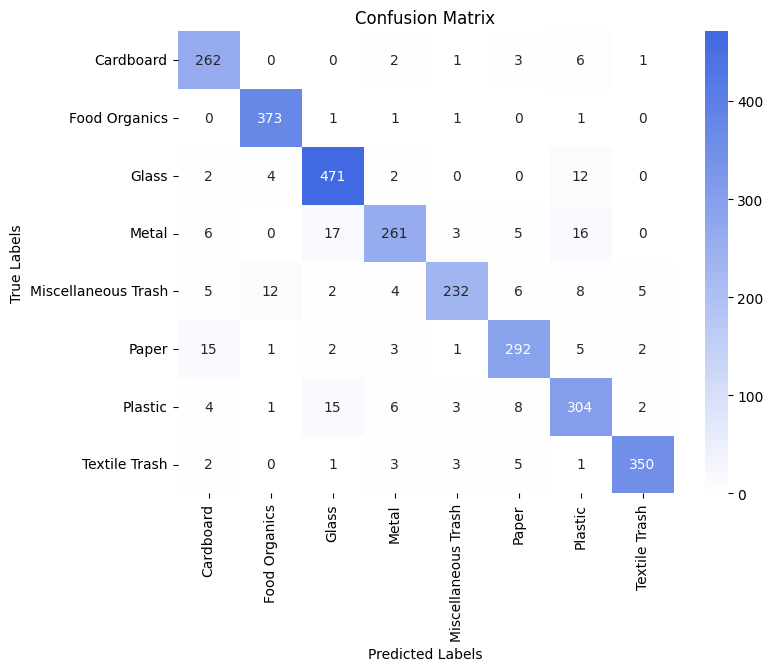
Test Accuracy: 92.41%

As the confusion matrix shows, metal trash is misclassified more often than the other labels. This suggests that the model still struggles to distinguish metal from certain classes, especially Glass and Plastic, possibly due to similarities in texture.

Conclusions

In this project, we successfully built an image classification model for waste sorting using transfer learning. After doing several optimization steps, the final model reached an accuracy of 92.41%, which met our project target. The model still struggles with certain classes (like metal), but overall, it performs well enough for deployment in an Android application.

What I Learned

Throughout this project, I learned a lot about the end to end process of building a machine learning model, including:

1. how to prepare and balance image datasets
2. how to apply transfer learning and fine tune pretrained models
3. how to experiment with different architectures to improve performance
4. how to evaluate a model properly using metrics

This project also taught me the importance of teamwork across different learning paths and how to communicate technical decisions clearly.

‍